Convergence checks
In this notebook we look at the adsorption energy and height of a nitrogen atom on a Ru(0001) surface in the hcp site. We check for convergence with respect to:
number of layers
number of k-points in the BZ
plane-wave cutoff energy
Nitrogen atom
First step is an isolated nitrogen atom which has a magnetic moment of 3.
More information:
ase.Atoms and GPAW parameters.
from ase import Atoms
from gpaw import GPAW, PW

ecut = 400.0
vacuum = 4.0

nitrogen = Atoms('N', magmoms=[3])
nitrogen.center(vacuum=4.0)
nitrogen.calc = GPAW(txt='n.txt',
                     mode=PW(ecut),
                     xc='PBE')
en = nitrogen.get_potential_energy()
print(en, 'eV')
Clean slab
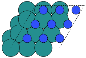
We use the ase.build.hcp0001() function to build the Ru(0001) surface.
from ase.build import hcp0001

nlayers = 2
a = 2.72
c = 1.58 * a

slab = hcp0001('Ru', a=a, c=c, size=(1, 1, nlayers), vacuum=vacuum)
from ase.visualize import view
view(slab, repeat=(3, 3, 2))

nkpts = 7
slab.calc = GPAW(txt='ru.txt',
                 mode=PW(ecut),
                 kpts={'size': (nkpts, nkpts, 1), 'gamma': True},
                 xc='PBE')
eru = slab.get_potential_energy()
N/Ru(0001)
Now, let’s add a nitrogen atom in the “HCP” site:
height = 1.1
nslab = hcp0001('Ru', a=a, c=c, size=(1, 1, nlayers))
# Calculate the coordianates of the N-atoms:
z = slab.positions[:, 2].max() + height
x, y = [2 / 3, 2 / 3] @ nslab.cell[:2, :2]
nslab.append('N')
nslab.positions[-1] = [x, y, z]
nslab.center(vacuum=vacuum, axis=2)  # 2: z-axis
view(nslab, repeat=(3, 3, 2))
Alternatively, you can just use the
ase.build.add_adsorbate() function:
from ase.build import add_adsorbate
add_adsorbate(nslab, 'N', position='hcp', height=height)
Now, calculate the total energy and the unrelaxed adsorption energy:
nslab.calc = GPAW(txt='nru.txt',
                  mode=PW(ecut),
                  poissonsolver={'dipolelayer': 'xy'},
                  kpts={'size': (nkpts, nkpts, 1), 'gamma': True},
                  xc='PBE')
enru0 = nslab.get_potential_energy()
print('Unrelaxed adsoption energy:', enru0 - eru - en, 'eV')

f = nslab.get_forces()
print(f[-1])
If you also calculate for forces (f = nslab.get_forces()),
you will see that the force on the N-atom is quite big (print(f[-1])).
Let’s freeze the surface and relax the
adsorbate. We use
ase.optimize.BFGSLineSearch and
ase.constraints.FixAtoms
for this task.
from ase.constraints import FixAtoms
from ase.optimize import BFGSLineSearch

nslab.constraints = FixAtoms(indices=list(range(nlayers)))
optimizer = BFGSLineSearch(nslab, trajectory='NRu.traj')
optimizer.run(fmax=0.01)
height = nslab.positions[-1, 2] - nslab.positions[:-1, 2].max()
print('Height:', height, 'Ang')
enru = nslab.get_potential_energy()
print('Relaxed adsorption energy:', enru - eru - en, 'eV')
Convergence
In order to make it easy to check for convergence of the adsorption energy
and height we write functions (called adsorp() and atom_energy())
that does all of the stuff above taking
nlayers, nkpts and ecut as input parameters.
Take a look at the convergence.py script and try to
understand what it does:
# web-page: results.json
import json
from pathlib import Path

from ase import Atoms
from ase.build import hcp0001
from ase.constraints import FixAtoms
from ase.optimize import BFGSLineSearch
from gpaw import GPAW, PW
from gpaw.mpi import world

a = 2.72
c = 1.58 * a
vacuum = 4.0


def adsorb(height: float = 1.2,
           nlayers: int = 3,
           nkpts: int = 7,
           ecut: float = 400) -> tuple[float, float, float]:
    """Adsorb nitrogen in hcp-site on Ru(0001) surface.

    Do calculations for N/Ru(0001), Ru(0001) and a nitrogen atom
    if they have not already been done.

    height: float
        Height of N-atom above top Ru-layer.
    nlayers: int
        Number of Ru-layers.
    nkpts: int
        Use a (nkpts * nkpts) Monkhorst-Pack grid that includes the
        Gamma point.
    ecut: float
        Cutoff energy for plane waves.

    Returns height, energy of N/Ru(0001) and clean Ru(0001).
    """

    name = f'Ru{nlayers}-{nkpts}x{nkpts}-{ecut:.0f}'

    parameters = dict(
        mode=PW(ecut),
        poissonsolver={'dipolelayer': 'xy'},
        kpts={'size': (nkpts, nkpts, 1), 'gamma': True},
        xc='PBE')

    # N/Ru(0001):
    slab = hcp0001('Ru', a=a, c=c, size=(1, 1, nlayers))
    z = slab.positions[:, 2].max() + height
    x, y = [2 / 3, 2 / 3] @ slab.cell[:2, :2]
    slab.append('N')
    slab.positions[-1] = [x, y, z]
    slab.center(vacuum=vacuum, axis=2)  # 2: z-axis

    # Fix first nlayer atoms:
    slab.constraints = FixAtoms(indices=list(range(nlayers)))

    slab.calc = GPAW(txt=f'N{name}.txt',
                     **parameters)
    optimizer = BFGSLineSearch(slab, logfile=f'N{name}.opt')
    optimizer.run(fmax=0.01)
    height = slab.positions[-1, 2] - slab.positions[:-1, 2].max()
    enru = slab.get_potential_energy()

    # Clean surface (single point calculation):
    del slab[-1]  # remove nitrogen atom
    slab.calc = GPAW(txt=f'{name}.txt',
                     **parameters)
    eru = slab.get_potential_energy()

    return height, enru, eru


def atom_energy(ecut: float = 400) -> float:
    """Calculate energy of spin-polarized nitrogen atom."""
    molecule = Atoms('N', magmoms=[3])
    molecule.center(vacuum=4.0)
    parameters = dict(
        mode=PW(ecut),
        xc='PBE')
    name = f'N-{ecut:.0f}'
    molecule.calc = GPAW(txt=f'{name}.txt', **parameters)
    en = molecule.get_potential_energy()
    return en


def main():
    h = 1.2  # initial guess

    # N-atom energies:
    eatom = {}
    for ecut in range(350, 801, 50):
        en = atom_energy(ecut)
        eatom[ecut] = en

    # Collect (layers, k-points, ecut, height, adsorption energy)
    # tuple in a list:
    results: list[tuple[int, int, int, float, float]] = []

    # ecut convergence:
    for ecut in range(350, 801, 50):
        h, enru, eru = adsorb(h, 2, 7, ecut)
        results.append((2, 7, ecut, h, enru - eru - eatom[ecut]))

    # Number of layers convergence:
    for n in range(1, 10):
        if n == 2:
            continue  # already done
        h, enru, eru = adsorb(h, n, 7, 400)
        results.append((n, 7, 400, h, enru - eru - eatom[ecut]))

    # Number of k-points convergence:
    for k in range(4, 18):
        if k == 7:
            continue  # already done
        h, enru, eru = adsorb(h, 2, k, 400)
        results.append((2, k, 400, h, enru - eru - eatom[ecut]))

    if world.rank == 0:
        Path('results.json').write_text(
            json.dumps(results, indent=1))


if __name__ == '__main__':
    main()
If you run the script, the main() function will run and all the
convergence calculations will be run. You can run the script yourself or
you can just download the results here: results.json. We will
now analyse the results.
Try this:
from matplotlib import pyplot as plt
from pathlib import Path
import json

results = json.loads(Path('results.json').read_text())
heights = {}
eads = {}
for n, k, ecut, h, e in results:
    heights[(n, k, ecut)] = h
    eads[(n, k, ecut)] = e

N = range(1, 10)
h = [heights[(n, 7, 400)] for n in N]
ea = [eads[(n, 7, 400)] for n in N]
fig, axs = plt.subplots(2, 1, sharex=True)
fig.subplots_adjust(hspace=0)
axs[0].plot(N, h)
axs[1].plot(N, ea)
axs[0].set_ylabel('height [Å]')
axs[1].set_ylabel('ads. energy [eV]')
axs[1].set_xlabel('number of layers')
# plt.show()
This should produce this:

Here are the plots for k-point and \(E_{text{cut}}\) convergence:


Conclusion
For accurate calculations you would need:
a plane-wave cutoff of 600 eV
5 layers of Ru
9x9 Monkhorst-Pack grid for BZ sampling (for a 1x1 unit cell)
For our quick’n’dirty calculations we will use 350 eV, 2 layers and a 4x4 \(\Gamma\)-centered Monkhorst-Pack grid (for a 2x2 unit cell).