Li intercalation energy in graphite
The Li intercalation energy in graphite page will guide you through the first day of the battery exercise.
Setup a graphite structure
Calculate C-C and interlayer distances
Use an empirical potential and DFT with a couple of exchange correlation functionals and compare with experimental values
Setup and calculate the energy of Li metal
Using DFT only from now on
Setup and calculate the combined structure of Li between graphene layers
Use all values to determine the Li intercalation energy
Compare the results of different functionals with experimental values.
Day 2 - Li intercalation energy
Today we will calculate the energy cost/gain associated with intercalating a lithium atom into graphite using approaches at different levels of theory. After today you should be able to:
Setup structures and do relaxations using ASE and GPAW.
Discuss which level of theory is required to predict the Li intercalation energy and why?
The Li intercalation reaction is:
and the intercalation energy will then be
Where \(x\) is the number of Carbon atoms in your computational cell.
We will calculate these energies using Density Functional Theory (DFT) with different exchange-correlation functionals. Graphite is characterised by graphene layers with strongly bound carbon atoms in hexagonal rings and weak long-range van der Waals interactions between the layers.
In the sections below we will calculate the lowest energy structures of each compound. This is needed to determine the intercalation energy.
Graphite
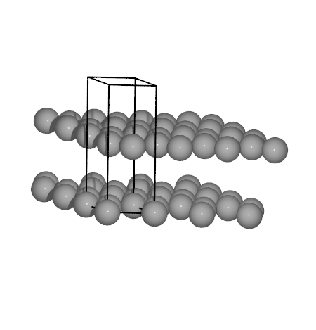
To try some of the methods that we are going to use we will start out by
utilizing the interatomic potential
emt (Effective Medium
Theory) calculator. This will allow to quickly test some of the
optimization procedures in ASE, and ensure that the scripts do what they
are supposed to, before we move on to the more precise and time
consuming DFT calculations. Initially we will calculate the C-C
distance and interlayer spacing in graphite in a two step procedure.
# The graphite structure is set up using a tool in ASE
from ase.lattice.hexagonal import Graphite

# One has only to provide the lattice constants
structure = Graphite('C', latticeconstant={'a': 1.5, 'c': 4.0})
To verify that the structures is as expected we can check it visually.
from ase.visualize import view
view(structure)  # This will pop up the ase gui window
Next we will use the EMT calculator to get the energy of graphite. Remember absolute energies are not meaningful, we will only use energy differences.
from ase.calculators.emt import EMT

calc = EMT()
structure.calc = calc
energy = structure.get_potential_energy()
print(f'Energy of graphite: {energy:.2f} eV')
Energy of graphite: 15.84 eV
The cell below requires some input. We set up a loop that should calculate the energy of graphite for a series of C-C distances.
import numpy as np

# Provide some initial guesses on the distances
ccdist = 1.3
layerdist = 3.7

# We will explore distances around the initial guess
dists = np.linspace(ccdist * .8, ccdist * 1.2, 10)
# The resulting energies are put in the following list
energies = []
for cc in dists:
    # Calculate the lattice parameters a and c from the C-C distance
    # and interlayer distance, respectively
    a = cc * np.sqrt(3)
    c = 2 * layerdist

    gra = Graphite('C', latticeconstant={'a': a, 'c': c})

    # Set the calculator and attach it to the Atoms object with
    # the graphite structure
    calc = EMT()
    gra.calc = calc

    energy = gra.get_potential_energy()
    # Append results to the list
    energies.append(energy)
Determine the equilibrium lattice constant. We use a
numpy.polynomial.
# Fit a polynomial:
poly = np.polynomial.Polynomial.fit(dists, energies, 3)
# and plot it:
# magic: %matplotlib notebook
import matplotlib.pyplot as plt
fig, ax = plt.subplots(1, 1)
ax.plot(dists, energies, '*r')
x = np.linspace(1, 2, 100)
ax.plot(x, poly(x))
ax.set_xlabel('C-C distance [Ang]')
ax.set_ylabel('energy [eV]')
poly1 = poly.deriv()
poly1.roots()  # two extrema
# Find the minimum:
emin, ccdist = min((poly(d), d) for d in poly1.roots())
print(f'C-C dist: {ccdist:.3f} Å')
# alternatively:
poly2 = poly1.deriv()
for ccdist in poly1.roots():
    if poly2(ccdist) > 0:
        break
print(f'C-C dist: {ccdist:.3f} Å')
from pathlib import Path
C-C dist: 1.319 Å
C-C dist: 1.319 Å
Make a script that calculates the interlayer distance with EMT in the cell below
# This script will calculate the energy of graphite
# for a series of inter-layer distances.
from ase.calculators.emt import EMT
from ase.lattice.hexagonal import Graphite
import numpy as np

# ccdist is already defined in the previous cell
# Start from a small guess
layerdist = 2.0
...
Now both the optimal C-C distance and the interlayer distance is evaluated with EMT. Try to compare with the experimental numbers provided below.
Experimental values |
EMT |
LDA |
PBE |
PBE+DFTD3 |
|
|---|---|---|---|---|---|
C-C distance / Å |
1.42 |
||||
Interlayer distance / Å |
3.35 |
Not surprisingly we need to use more sophisticated theory to model this issue. Below we will use DFT as implemented in GPAW to determine the same parameters.
First we set up an initial guess of the structure as before.
import numpy as np
from ase.lattice.hexagonal import Graphite
from gpaw import GPAW, PW
from ase.filters import StrainFilter
from ase.optimize.bfgs import BFGS

ccdist = 1.40
layerdist = 3.33
a = ccdist * np.sqrt(3)
c = 2 * layerdist
gra = Graphite('C', latticeconstant={'a': a, 'c': c})
Then we create the GPAW calculator object. The parameters are explained
here,
see especially the section regarding
Plane-wave, LCAO or Finite-difference mode?.
This graphite structure has a small unit cell, thus plane wave mode,
mode=PW(), will be faster than the grid mode, mode='fd'. Plane wave
mode also lets us calculate the strain on the unit cell - useful for
optimizing the lattice parameters.
We will start by using the LDA exchange-correlation functional. Later you will try other functionals.
# web-page: graphite-LDA.traj, graphite-LDA.txt
import numpy as np
from ase.lattice.hexagonal import Graphite
from gpaw import GPAW, PW
from ase.filters import StrainFilter
from ase.optimize.bfgs import BFGS

ccdist = 1.40
layerdist = 3.33
a = ccdist * np.sqrt(3)
c = 2 * layerdist
gra = Graphite('C', latticeconstant={'a': a, 'c': c})

xc = 'LDA'
calcname = f'graphite-{xc}'
calc = GPAW(mode=PW(500),
            kpts=(10, 10, 6),
            xc=xc,
            txt=calcname + '.txt')
gra.calc = calc  # Connect system and calculator
print(gra.get_potential_energy())
Check out the contents of the output file (graphite-LDA.txt),
all relevant information about the scf cycle are printed therein.
Then we optimize the unit cell of the structure. We will take advantage
of the ase.filters.StrainFilter
class. This allows us to simultaneously optimize both C-C distance and
interlayer distance. We employ the
BFGS algorithm to
minimize the strain on the unit cell.
sf = StrainFilter(gra, mask=[1, 1, 1, 0, 0, 0])
opt = BFGS(sf, trajectory=calcname + '.traj', logfile=calcname + '.log')
opt.run(fmax=0.01)
Read in the result of the relaxation and determine the C-C and interlayer distances.
from ase.io import read
import numpy as np

atoms = read('graphite-LDA.traj')
# or
atoms = read('graphite-LDA.txt')
a = atoms.cell[0, 0]
h = atoms.cell[2, 2]
# Determine the rest from here
print(f'C-C: {a / np.sqrt(3):.3f} Å')
print(f'layer-distance: {h / 2:.3f} Å')
C-C: 1.411 Å
layer-distance: 3.213 Å
Now we need to try a GGA type functional (e.g. PBE) and also try to add van der Waals forces on top of PBE (i.e. PBE+DFTD3). These functionals will require more computational time, thus the following might be beneficial to read.
If the relaxation takes too long time, we can submit it to be run in parallel on the computer cluster. Remember we can then run different calculations simultaneously.
Log in to the gbar terminal, save a full script in a file
(e.g. \(calc.py\)) and submit that file to be calculated in parallel
(e.g. mq submit calc.py -R 8:1h (1 hour on 8 cores)).
Note
Read more about MyQueue here: https://myqueue.readthedocs.io/
Check the status of the calculation by mq ls.
When the calculation finishes the result can be interpreted by
using the ASE read() function to get an atoms
object. This assumes that the trajectory file is called:
graphite-LDA.traj, if not change accordingly.
from ase.io import read
# The full relaxation
relaxation = read('graphite-LDA.traj', index=':')
# The final image of the relaxation containing the relevant energy
atoms = read('graphite-LDA.traj')
# Extract the relevant information from the calculation
# Energy
energy = atoms.get_potential_energy()

# Unit cell
cell = atoms.get_cell()

# See the steps of the optimization
from ase.visualize import view
view(relaxation)
Li metal
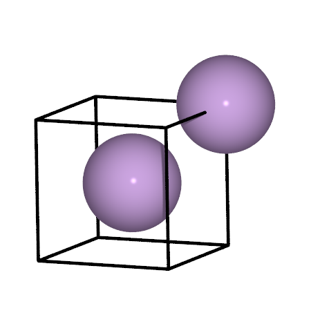
Now we need to calculate the energy of Li metal. We will use the same strategy as for graphite, i.e. first determine the lattice constant, then use the energy of that structure. This time though you will have to do most of the work.
Some hints:
The crystal structure of Li metal is shown in the image above. That structure is easily created with one of the functions in the
ase.buildmoduleA k-point density of approximately 2.4 points / Angstrom will be sufficient
The DFTD3 correction is done a posteriori, this means the calculator should be created a little differently, see [the second example here](https://ase-lib.org/ase/calculators/dftd3.html#examples)
See also the
equation of state module
In the end try to compare the different functionals with experimental values:
Experimental values |
LDA |
PBE |
PBE+DFTD3 |
|
|---|---|---|---|---|
a / Å |
3.51 |
Li intercalation in graphite
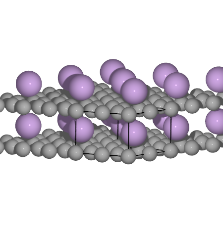
Now we will calculate the intercalation of Li in graphite. For simplicity we will represent the graphite with only one layer. Also try and compare the C-C and interlayer distances to experimental values.
Experimental values |
LDA |
PBE |
PBE+DFTD3 |
|
|---|---|---|---|---|
C-C distance / Å |
1.441 |
|||
Interlayer distance / Å |
3.706 |
# A little help to get you started with the combined structure
from ase.lattice.hexagonal import Graphene
from ase import Atom

# We will have to optimize these distances
ccdist = 1.40
layerdist = 3.7

a = ccdist * np.sqrt(3)
c = layerdist

# We will require a larger cell, to accomodate the Li
Li_gra = Graphene('C', size=(2, 2, 1), latticeconstant={'a': a, 'c': c})
# Append an Li atom on top of the graphene layer
Li_gra.append(Atom('Li', (a / 2, ccdist / 2, layerdist / 2)))
Now calculate the intercalation energy of Li in graphite with the following formula:
where \(x\) is the number of Carbon atoms in your Li intercalated graphene cell. Remember to adjust the energies so that the correct number of atoms is taken into account.
These are the experimental values to compare with In the end try to compare the different functionals with experimental values:
Experimental values |
LDA |
PBE |
PBE+DFTD3 |
|
|---|---|---|---|---|
Intercalation energy / eV |
-0.124 |
Great job! When you have made it this far it is time to turn your attention to the cathode. If you have lots of time left though see if you can handle the bonus exercise.
Bonus
In the calculation of the intercalated Li we used a graphene layer with 8 Carbon atoms per unit cell. We can actually use only 6 Carbon by rotating the x and y cell vectors. This structure will be faster to calculate and still have neglible Li-Li interaction.
from ase import Atoms

ccdist = 1.40
layerdist = 3.7

a = ccdist * np.sqrt(3)
c = layerdist

Li_gra = Atoms('C6Li')  # Fill out the positions and cell vectors
...