Catalysis: Dissociative adsorption of N₂ on a metal surface

This is the rate limiting step for ammonia synthesis.

Scientific disclaimer: These calculations are done on a flat surface. In reality, the process takes place at the foot of an atomic step on the surface. Doing calculations on this more realistic system would be too slow for these exercises. For the same reason, we use a metal slab with only two layers, a realistic calculation would require the double.

N₂ Adsorption on a metal surface

This tutorial shows how to calculate the adsorption energy of an N₂ molecule on a closepacked Ru surface. The first cell imports some modules from the ASE and GPAW packages

from ase import Atoms
from gpaw import GPAW, PW
from ase.constraints import FixAtoms
from ase.optimize import QuasiNewton
from ase.build import hcp0001
from ase.visualize import view
from ase.io import read, write
import time

Setting up the metal surface

Ru crystalises in the hcp structure with a lattice constants a = 2.706 Å and c = 4.282 Å. It is often better to use the lattice constants corresponding to the DFT variant used (here PBE with PAW). We get this from https://oqmd.org.

We model the surface by a 2 layer slab of metal atoms, and add 5Å vacuum on each side.

We visualize the system with ASE GUI, so you can check that everything looks right. This pops up a new window.

a_Ru = 2.704  # PBE value from OQMD.org; expt value is 2.706
slab = hcp0001('Ru', a=a_Ru, size=(2, 2, 2), vacuum=5.0)

# Other metals are possible, for example Rhodium
# Rhodium is FCC so you should use fcc111(...) to set up the system
# (same arguments).
# Remember to set the FCC lattice constant, get it from OQMD.org.

# a_Rh = 3.793
# slab = fcc111('Rh', a=a_Rh, size=(2, 2, 2), vacuum=5.0)

view(slab)

To optimise the slab we need a calculator. We use the GPAW calculator in plane wave (PW) mode with the PBE exchange—correlation functional. The convergence with respect to the cutoff energy and k-point sampling should always be checked — see Convergence checks for more information on how this can be done. For this exercise an energy cutoff of 350eV and 4x4x1 k-point mesh is chosen to give reasonable results with a limited computation time.

calc = GPAW(xc='PBE',
            mode=PW(350),
            kpts={'size': (4, 4, 1), 'gamma': True},
            convergence={'eigenstates': 1e-6})
slab.calc = calc

The bottom layer of the slab is fixed during optimisation. The structure is optimised until the forces on all atoms are below 0.05 eV/Å.

z = slab.positions[:, 2]
constraint = FixAtoms(mask=(z < z.min() + 1.0))
slab.set_constraint(constraint)
dyn = QuasiNewton(slab, trajectory='Ru.traj')
t = time.time()
dyn.run(fmax=0.05)
print(f'Wall time: {(time.time() - t) / 60} min.')

The calculation will take ca. 5 minutes. While the calculation is running you can take a look at the output. How many k-points are there in total and how many are there in the irreducible part of the Brillouin zone? What does this mean for the speed of the calculation?

What are the forces and the energy after each iteration? You can read it directly in the output above, or from the saved .traj file like this:

iter0 = read('Ru.traj', index=0)
print('Energy: ', iter0.get_potential_energy())
print('Forces: ', iter0.get_forces())

Often you are only interested in the final energy which can be found like this:

e_slab = slab.get_potential_energy()
print(e_slab)

Making a Nitrogen molecule

We now make an N₂ molecule and optimise it in the same unit cell as we used for the slab.

d = 1.10
molecule = Atoms('2N', positions=[(0., 0., 0.), (0., 0., d)])
molecule.set_cell(slab.get_cell())
molecule.center()
calc_mol = GPAW(xc='PBE', mode=PW(350))
molecule.calc = calc_mol
dyn2 = QuasiNewton(molecule, trajectory='N2.traj')
dyn2.run(fmax=0.05)
e_N2 = molecule.get_potential_energy()

We can calculate the bond length like this:

d_N2 = molecule.get_distance(0, 1)
print(d_N2)

How does this compare with the experimental value?

Adsorbing the molecule

Now we adsorb the molecule on top of one of the Ru atoms.

Here, it would be natural to just add the molecule to the slab, and minimize. However, that takes 45 minutes to an hour to converge, so we cheat to speed up the calculation.

The main slowing-down comes from the relaxation of the topmost metal atom where the N₂ molecule binds, this atom moves a quarter of an Ångström out. Also, the binding length of the molecule changes when it is adsorbed, so we build a new molecule with a better starting guess.

h = 1.9  # guess at the binding height
d = 1.2  # guess at the binding distance
slab.positions[4, 2] += 0.2  # pre-relax the binding metal atom.

molecule = Atoms('2N', positions=[(0, 0, 0), (0, 0, d)])
p = slab.get_positions()[4]
molecule.translate(p + (0, 0, h))
slabN2 = slab + molecule
constraint = FixAtoms(mask=(z < z.min() + 1.0))
slabN2.set_constraint(constraint)
view(slabN2)

We optimise the structure. Since we have cheated and have a good guess for the initial configuration we prevent that the optimization algorithm takes too large steps.

slabN2.calc = calc
dyn = QuasiNewton(slabN2, trajectory='N2Ru-top.traj', maxstep=0.02)
t = time.time()
dyn.run(fmax=0.05)
print(f'Wall time: {(time.time() - t) / 60} min.')

The calculation will take a while (10-15 minutes). While it is running please follow the guidelines in the Exercise section below.

Once the calculation is finished we can calculate the adsorption energy as: \(E_{\mathrm{ads}} = E_{\mathrm{slab+N}_2} - (E_{\mathrm{slab}} + E_{\mathrm{N}_2})\).

print('Adsorption energy:', slabN2.get_potential_energy() - (e_slab + e_N2))

Try to calculate the bond length of N₂ adsorbed on the surface. Has it changed? What is the distance between the N₂ molecule and the surface?

Exercise

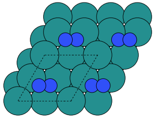
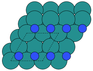
1. Make a script and set up an adsorption configuration where the N₂ molecule is lying down with the center of mass above a three-fold hollow site as shown below. Use an adsorption height of 1.7 Å.

Remember that you can read in the \(traj\) files you have saved, so you don’t need to optimise the surface again.

View the combined system before you optimize the structure to ensure that you created what you intended.

slab = read('Ru.traj')
view(slab)

Note that when viewing the structure, you can find the index of the individual atoms in the slab object by clicking on them.

You might also find the get_center_of_mass() and rotate() methods useful.

Now you should optimize the structure as you did before with the N₂ molecule standing. The calculation will probably bee too long to run interactively. Prototype it in the terminal, then interrupt the calculation.

Check the number of irreducible k-points and then submit the job as a batch job running on that number of CPU cores.

3. Make a configuration where two N atoms are adsorbed in hollow sites on the surface as shown below

Note that here the two N atoms sit on next-nearest hollow sites. An alternative would be to have them on nearest neighbor sites. If you feel energetic you could investigate that as well. Also, there are two different kinds of hollow sites, they are not completely equivalent!

Optimise the structure and get the final energy. Is it favourable to dissociate N₂ on the surface? What is the N—N distance now? What does that mean for catalysis?