Using the BSE+ method

In this tutorial, we calculate the BSE+ [1] q-resolved electron energy loss spectrum (q-EELS) of TiO2 and MoS2, as well as the refractive index for TiO2.

Absorption spectrum of TiO2

BSE+ needs two kinds of ground state gpw-files as input. One with fewer k-points to calculate the BSE, and one with more k-points and bands for the RPA calculations.

The files created will be called fixed_density_calc_TiO2_bse.gpw which will contain fewer k-points for the BSE calculation itself. Note, that BSE calculation will require many bands to calculate the screened interaction W, which demands a significant number of unoccupied bands.

The second file, fixed_density_calc_TiO2_rpa.gpw, will contain even more bands for the RPA calculation and a higher k-point density to ensure better convergence.

This calculation will run 20mins with 80 cores.

from gpaw import GPAW
from gpaw import PW
from gpaw.occupations import FermiDirac
from ase.spacegroup import crystal

aa = 4.584
c = 2.953

a = crystal(['Ti', 'O'], basis=[(0, 0, 0), (0.3, 0.3, 0.0)],
            spacegroup=136, cellpar=[aa, aa, c, 90, 90, 90])

name_calc = 'calc_TiO2_BSEPlus'
name_bse_plus = 'fixed_density_calc_TiO2_bse'
name_rpa = 'fixed_density_calc_TiO2_rpa'

calc = GPAW(mode=PW(800),
            xc='PBE',
            occupations=FermiDirac(width=0.01),
            parallel={'domain': 1, 'band': 1},
            convergence={'bands': 50, 'density': 1e-4,
                         'eigenstates': 4e-07, 'energy': 5e-4},
            kpts={'density': 8, 'gamma': True, 'even': True})
a.calc = calc
a.get_potential_energy()
calc.write(name_calc + ".gpw")

calc_es = GPAW(name_calc + '.gpw').fixed_density(
    convergence={'bands': 50},
    nbands=60, parallel={'domain': 1},
    kpts={'density': 6, 'gamma': True, 'even': True})
calc_es.diagonalize_full_hamiltonian(nbands=100)
calc_es.write(name_bse_plus + '.gpw', mode='all')

calc_es = GPAW(name_calc + '.gpw').fixed_density(
    convergence={'bands': 100},
    nbands=240, parallel={'domain': 4},
    kpts={'density': 15, 'gamma': True, 'even': True})
calc_es.write(name_rpa + '.gpw', mode='all')

Now we are ready to perform the actual BSE+ calculation. We instantiate the BSEPlus object, which requires these two gpw-files: one for the BSE calculation, and one for the RPA calculation. Parameters starting with bse_ are related to the BSE calculation, and should be se as in a standard BSE calculation. We use 60 bands to calculate the screening (W) for BSE, and 130 bands for the RPA calculation. We shift the bandgap to match the direct band gap of TiO2, aligning the lowest peak observed in the refractive index calculated with BSE with the lowest peak in the refractive index observed in the experimental data.

This calculation will run 2 hours with 80 cores.

from gpaw import GPAW
import numpy as np
from gpaw.response.bse import BSEPlus
from ase.dft.bandgap import bandgap

calc_bse = 'fixed_density_calc_TiO2_bse.gpw'
calc_rpa = 'fixed_density_calc_TiO2_rpa.gpw'

ecut = 80
eta = 0.1
q_c = [0.0, 0.0, 0.0]
bse_valence_bands = range(18, 24)
bse_conduction_bands = range(24, 30)
bse_nbands = 60
rpa_nbands = 130
w_w = np.linspace(0, 50, 5001)

gap, _, _ = bandgap(GPAW(calc_rpa), direct=True)
eshift = 3.3 - gap

bseplus = BSEPlus(bse_gpw=calc_bse,
                  bse_valence_bands=bse_valence_bands,
                  bse_conduction_bands=bse_conduction_bands,
                  bse_nbands=bse_nbands,
                  rpa_gpw=calc_rpa,
                  rpa_nbands=rpa_nbands,
                  w_w=w_w,
                  eshift=eshift,
                  eta=eta,
                  q_c=q_c,
                  ecut=ecut)

bseplus.calculate_chi_wGG(optical=True,
                          bsep_name='chi_TiO2_BSEPlus',
                          save_chi_BSE='chi_TiO2_BSE',
                          save_chi_RPA='chi_TiO2_RPA')

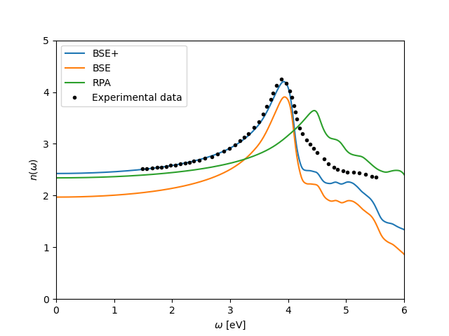
Now we can plot the results together with the experimental data which can be downloaded from here tio2_n_rutile_inplane.csv [2], eels_tio2_rutile.csv [3].

import matplotlib.pyplot as plt
import numpy as np


def refractive_index(chi):
    eps = 1 + np.pi * 4 * chi
    eps1 = eps.real
    eps2 = eps.imag
    N = np.sqrt(0.5 * (np.sqrt(eps1**2 + eps2**2) + eps1))
    return N


def eels(chi):
    eps = np.pi * 4 * chi + 1
    return (-eps**(-1)).imag


chi_bsep = np.load('chi_TiO2_BSEPlus.npy')
chi_bse = np.load('chi_TiO2_BSE.npy')
chi_rpa = np.load('chi_TiO2_RPA.npy')
x = np.linspace(0, 50, 5001)

exp_data = np.loadtxt('tio2_n_rutile_inplane.csv', delimiter=',')
freq = exp_data[:, 0]
exp_n = exp_data[:, 1]

n_bsep = refractive_index(-chi_bsep[:, 0, 0])
n_bse = refractive_index(-chi_bse[:, 0, 0])
n_rpa = refractive_index(-chi_rpa[:, 0, 0])

plt.plot(x, n_bsep, label='BSE+')
plt.plot(x, n_bse, label='BSE')
plt.plot(x, n_rpa, label='RPA')
plt.plot(freq, exp_n, '.', color='black', label='Experimental data')

plt.legend()
plt.xlabel(r'$\omega$' + ' [eV]')
plt.ylabel(r'$n(\omega)$')
plt.xlim(0, 6)
plt.ylim(0, 5)
plt.savefig('n_TiO2.png')
plt.close()

eels_bsep = eels(-chi_bsep[:, 0, 0])
eels_bse = eels(-chi_bse[:, 0, 0])
eels_rpa = eels(-chi_rpa[:, 0, 0])
exp_data = np.loadtxt('eels_tio2_rutile.csv', delimiter=',')
freq = exp_data[:, 0]
exp_eels = exp_data[:, 1]

plt.plot(x, eels_bsep, label='BSE+')
plt.plot(x, eels_bse, label='BSE')
plt.plot(x, eels_rpa, label='RPA')
plt.plot(freq, exp_eels * 40, '.', color='black', label='Experimental data')

plt.legend()
plt.xlabel('Energy [eV]')
plt.ylabel(r'$\mathrm{I}_\mathrm{EELS}$' + ' [arb. units]')
plt.xlim(0, 25)
plt.ylim(0, 1.2)
plt.savefig('eels_TiO2.png')

Absorption spectrum of MoS2

BSE+ can also be used to calculate q-EELS spectra of 2D materials. Here, we calculate the EELS for a slab of MoS2 at \(q=0.074 Ao^{-1}\).

As before, the files fixed_density_calc_MoS2_bse.gpw and fixed_density_calc_MoS2_rpa.gpw will be created with the former containing fewer k-points for the BSE calculation. The k-point densities are chosen such that the BSE k-point grid is contained in the RPA k-point grid to allow for finite q calculations.

This calculation will run 35mins with 80 cores and requires the structure file for MoS2 MoS2.json.

from gpaw import GPAW, PW, FermiDirac
from ase.build import mx2

slab = mx2('MoS2', kind='2H', a=3.1841, thickness=3.1271, vacuum=7.5)

name_calc = 'calc_MoS2_BSEPlus'
calc_bse = 'fixed_density_calc_MoS2_bse'
calc_rpa = 'fixed_density_calc_MoS2_rpa'

calc = GPAW(mode=PW(800),
            xc='PBE',
            nbands=200,
            convergence={'bands': -5, 'density': 1e-4,
                         'eigenstates': 4e-08, 'energy': 5e-5},
            occupations=FermiDirac(width=0.01),
            kpts={'density': 26, 'gamma': True},
            txt='gs_MoS2.txt')

slab.calc = calc
slab.get_potential_energy()
calc.write(name_calc + ".gpw")

calc_es = GPAW(name_calc + '.gpw').fixed_density(
    txt='bse_calc.txt',
    convergence={'bands': 50},
    nbands=100, parallel={'domain': 1},
    kpts={'density': 11.7, 'gamma': True})
calc_es.diagonalize_full_hamiltonian(nbands=100)
calc_es.write(calc_bse + '.gpw', mode='all')

calc_es = GPAW(name_calc + '.gpw').fixed_density(
    txt='rpa_calc.txt',
    convergence={'bands': 80, 'density': 1e-5,
                 'eigenstates': 4e-8, 'energy': 5e-5},
    nbands=220,
    kpts={'density': 23.5, 'gamma': True})
calc_es.write(calc_rpa + '.gpw', mode='all')

We are now ready to do the BSE+ calculation. This time, we use a truncated Coulomb kernel and include spin-orbit coupling in the BSE calculation.

This calculation will run 2 hours with 80 cores.

from gpaw import GPAW
from gpaw.response.bse import BSEPlus
import numpy as np
from ase.dft.bandgap import bandgap


calc_bse = 'fixed_density_calc_MoS2_bse.gpw'
calc_rpa = 'fixed_density_calc_MoS2_rpa.gpw'

ecut = 50
eta = 0.05
q_c = [0.07407407, 0.0, 0.0]
bse_valence_bands = range(18, 26)
bse_conduction_bands = range(26, 34)
bse_nbands = 100
rpa_nbands = 170
w_w = np.linspace(0, 50, 5001)

gap, _, _ = bandgap(GPAW(calc_rpa), direct=True)
eshift = 2.53 - gap

bseplus = BSEPlus(bse_gpw=calc_bse,
                  bse_valence_bands=bse_valence_bands,
                  bse_conduction_bands=bse_conduction_bands,
                  bse_nbands=bse_nbands,
                  rpa_gpw=calc_rpa,
                  rpa_nbands=rpa_nbands,
                  w_w=w_w,
                  eshift=eshift,
                  bse_add_soc=True,
                  eta=eta,
                  q_c=q_c,
                  truncation='2D',
                  ecut=ecut)

bseplus.calculate_chi_wGG(optical=False,
                          bsep_name='chi_MoS2_BSEPlus',
                          save_chi_BSE='chi_MoS2_BSE',
                          save_chi_RPA='chi_MoS2_RPA')

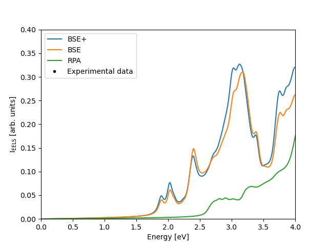
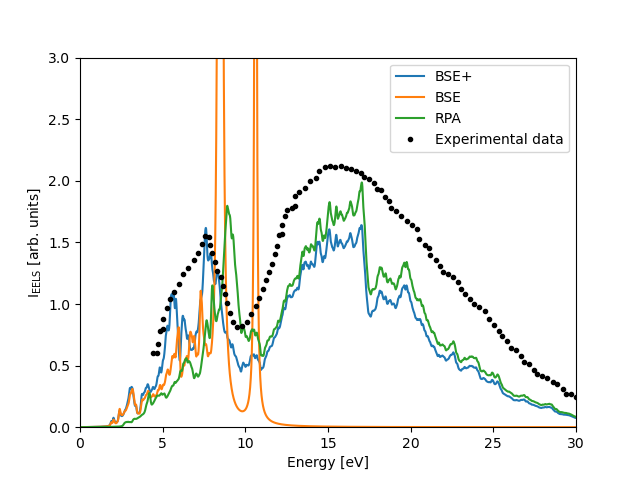
We can then plot the resulting EELS spectrum. We create two plots, one showing a broad frequency range and another zoomed in on the x-axis to visualize the spin-orbit-split exciton below the band edge. The results are shown together with the experimental data which can be downloaded from here MoS2_q_0p060Ainv.csv [4].

import matplotlib.pyplot as plt
import numpy as np


chi_bsep = np.load('chi_MoS2_BSEPlus.npy')
chi_bse = np.load('chi_MoS2_BSE.npy')
chi_rpa = np.load('chi_MoS2_RPA.npy')
x = np.linspace(0, 50, 5001)

data_high_w = np.loadtxt('MoS2_q_0p060Ainv.csv', delimiter=',')
w_high = data_high_w[:, 0]
eels_high = data_high_w[:, 1]

plt.plot(x, -chi_bsep[:, 0, 0].imag, label='BSE+')
plt.plot(x, -chi_bse[:, 0, 0].imag, label='BSE')
plt.plot(x, -chi_rpa[:, 0, 0].imag, label='RPA')
plt.plot(w_high, eels_high * 150, '.', color='black',
         label='Experimental data')

plt.legend()
plt.xlabel('Energy [eV]')
plt.ylabel(r'$\mathrm{I}_\mathrm{EELS}$' + ' [arb. units]')
plt.xlim(0, 30)
plt.ylim(0, 3)
plt.savefig('eels_MoS2.png')

plt.xlim(0, 4)
plt.ylim(0, 0.4)
plt.savefig('eels_MoS2_low_frequencies.png')

[1]

Søndersted et al. Phys. Rev. Lett. 133, 026403 (2024)

[2]

Jellison et al. J. Appl. Phys. 93, 9537 (2003)

[3]

Launay et al. Phys. Rev. B 69, 035101 (2004)

[4]

Köster et al. Micron 106, 103303 (2022)