Quasi-particle spectrum in the GW approximation from LCAO wave functions: tutorial

For a brief introduction to the GW theory and the details of its implementation in GPAW, see Quasi-particle spectrum in the GW approximation: theory.

More information can be found here:

F. Hüser, T. Olsen, and K. S. Thygesen

Quasiparticle GW calculations for solids, molecules, and two-dimensional materials

Physical Review B, Vol. 87, 235132 (2013)

Additionally, before getting started using LCAO wave functions in the GW approximation, it would be beneficial to become familiar with G0W0 using GPAW, see Quasi-particle spectrum in the GW approximation: tutorial.

Quasi-particle spectrum of bulk diamond

Groundstate LCAO calculation

First, we need to do a regular LCAO groundstate calculation, and save all of the wave functions. The basis-set is chosen using the basis keyword, and nbands is set to nao, reflecting the maximum nbands value that can be used in LCAO, which is the same number of bands as there are atomic orbitals.

from ase.build import bulk
from gpaw import GPAW, FermiDirac

a = 3.567
atoms = bulk('C', 'diamond', a=a)

calc = GPAW(mode='lcao',
            basis='dzp',
            kpts={'size': (8, 8, 8), 'gamma': True},
            xc='LDA',
            nbands='nao',
            occupations=FermiDirac(0.0),
            txt='C_lcao_groundstate.txt')

atoms.calc = calc
atoms.get_potential_energy()
calc.write('C_lcao_groundstate.gpw', mode='all')

G0W0 calculation using LCAO basis functions

We can now set up the G0W0 calculation similar to the PW case, passing the LCAO groundstate calculation C_lcao_groundstate.gpw to the G0W0 calculator, which is then internally converted to PW. However, there are a few major differences. ecut_extrapolation is disabled, because the convergence wrt. G-bands and chi0 bands is unknown with LCAO-basis set, whereas in PW mode, the number of bands can be just directly chosen from the plane wave cut off.

import numpy as np
from gpaw.dft import DFT
from gpaw.response.g0w0 import G0W0

dft = DFT.from_gpw_file('C_lcao_groundstate.gpw')
dft.change_mode('pw')
dft.write_gpw_file('C_pw_from_lcao_groundstate.gpw', include_wfs=True)

gw = G0W0('C_pw_from_lcao_groundstate.gpw',
          integrate_gamma='WS',
          ecut=200,
          nbands=26,
          kpts=[0],
          eta=0.1,
          bands=(3, 5),
          evaluate_sigma=np.linspace(-50, 75, 500),
          filename='C-g0w0-lcao')

gw.calculate()

The results are stored in C-g0w0-lcao_results.pckl.

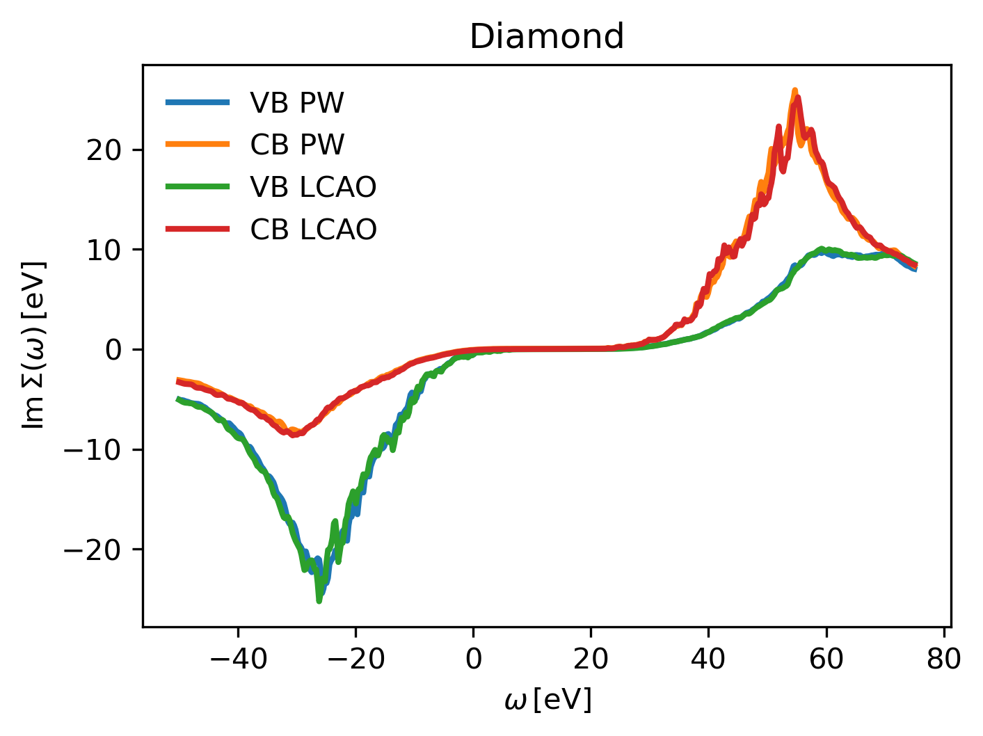
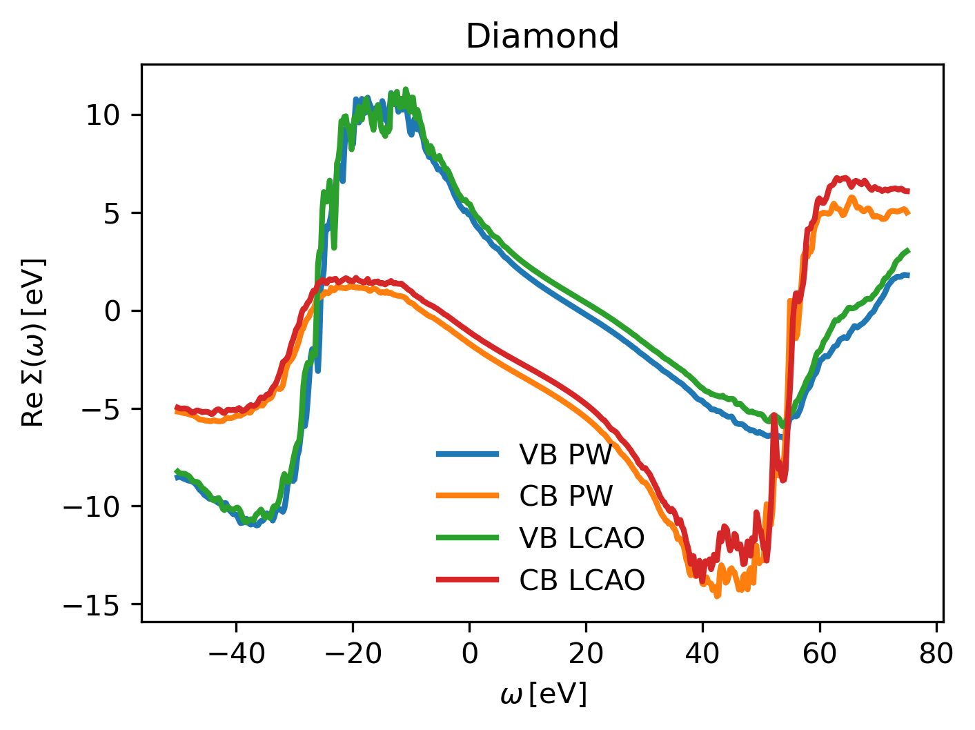
GW self-energy for Diamond (C)

We plot the results stored in C-g0w0-lcao_results.pckl as the imaginary and real part of the GW self-energy \(\Sigma(\omega)\) depending on the frequency using the script plot_C_lcao_gw.py. We compare the LCAO results to PW ones computed using C_pw_groundstate.py and C_pw_gw.py.